Beyond Volatility: A Quantitative Analysis of Portfolio Variance, Statistical Probabilities, and Advanced Risk Modeling
Deconstructing Portfolio Risk

This article provides a comprehensive analysis of portfolio risk, commencing with the foundational concept of “portfolio variation” and culminating in an expert-level critique of the statistical models that govern modern finance.
The central thesis of this analysis is twofold.
First, true portfolio risk is not a simple average of the risks of its constituent assets. Rather, portfolio risk is overwhelmingly dictated by the interaction between these assets, a concept quantified by covariance and correlation. This mathematical relationship is the fundamental engine of diversification, the only mechanism by which risk can be reduced without a corresponding sacrifice in expected return.
Second, the standard “Bell Curve” (Normal Distribution) and its associated standard deviation metrics, while representing the foundational tools of Modern Portfolio Theory, are critically flawed in practice. Real-world financial markets do not adhere to this clean, symmetrical distribution. Instead, they exhibit “fat tails“ (leptokurtosis), a statistical property which means that extreme, portfolio-destroying events (i.e., market crashes) are thousands of times more likely than the “normal” model predicts.
This article will execute the following analysis:
Define and derive the calculation for both single-asset volatility and multi-asset portfolio variance, the mathematical core of diversification.
Explain the role of the Bell Curve and the “68-95-99.7” Empirical Rule in the conventional translation of a volatility statistic into a probability of gain or loss.
Provide a complete, step-by-step guide to answer the core practical query: how to calculate the probable 1-day range of a portfolio’s movement, with both 1-standard-deviation and 2-standard-deviation probabilities.
Critically analyze the profound failures of this standard model, demonstrating why standard deviation is an incomplete, and often dangerously misleading, measure of true financial risk.
Introduce the professional-grade risk metrics that evolved to address these failures: Value at Risk (VaR) and its analytically superior, modern alternative, Conditional Value at Risk (CVaR), also known as Expected Shortfall.
The final deliverable is an exhaustive, rigorous, and nuanced research package designed to serve as a definitive quantitative foundation for understanding, calculating, and—most importantly—critiquing modern financial risk.
Part 1: The Bedrock of Risk – Variance and Volatility
This section establishes the fundamental language of risk. Before analyzing the variance of a portfolio, it is essential to first master the measurement of risk for a single asset.
1.1. Understanding Risk as Dispersion: Defining Variance and Volatility
In modern finance, risk is a quantifiable concept. Portfolio variance is a statistical value that measures the degree of dispersion of a portfolio’s returns around its expected (mean) return. It is a foundational concept in Modern Portfolio Theory (MPT).
This quantitative approach was revolutionary. Prior to the 1950s, investors assessed risk qualitatively, using financial reports or news events to form a “qualitative perception” of an asset’s future. Harry Markowitz, in his 1952 paper “Portfolio Selection,” provided the mathematical framework to quantify this risk.
MPT posits that a rational investor should not be concerned with risk in the abstract, but specifically with the statistical variance (represented as σ²) or its square root, the standard deviation (represented as σ).
The interpretation is straightforward:
A higher portfolio variance indicates greater volatility. This means the portfolio’s actual returns are likely to fluctuate wildly, deviating significantly from its long-term average. This implies higher risk.
A lower portfolio variance suggests more stable, predictable returns that are clustered tightly around the average. This implies lower risk.
The term volatility is the most common financial vernacular for standard deviation. It is the most widely used measure of investment risk.
The central premise of MPT is that investors are, or should be, “variance averse”. The entire goal of portfolio construction is to minimize this variance (risk) for any given level of expected return, or conversely, to maximize expected return for a given level of variance. The set of portfolios that achieve this balance is known as the “efficient frontier”.
Therefore, the query for “portfolio variation” is a query for the central variable that modern asset allocation seeks to minimize.
1.2. Variance (σ²) vs. Standard Deviation (σ): A Practical Comparison
While often used interchangeably in conversation, variance and standard deviation have a critical distinction that impacts their interpretability.
Variance (σ²): This is the average of the squared deviations from the mean.
Standard Deviation (σ): This is the square root of the variance.
The calculation of variance is a necessary mathematical step, but the resulting number is not intuitive. If an asset’s returns are measured in percent (%), its variance is measured in “percent-squared”. This squared unit is statistically correct but has no tangible, real-world meaning.
Standard deviation solves this problem. By taking the square root of the variance, σ is returned to the original units of the data. If the returns are in percent, the standard deviation is also in percent. This makes it directly interpretable.
For example, an annualized standard deviation of 15% on a portfolio with an average 10% return means that its returns (under a normal distribution) will typically fall in a range of 15 percentage points around that 10% average.
To calculate standard deviation, one must calculate variance first. Standard deviation is the final, interpretable output; variance is the necessary mathematical engine.
This engine has a critical feature: the act of squaring the deviations from the mean (the (R_i - μ)² term in the formula) gives disproportionately more weight to large deviations (outliers) than to small ones. A return that is 3 units from the mean adds 9 to the variance calculation, while a return that is 1 unit away adds only 1. This is a desirable feature, as it correctly identifies an asset with rare, wild swings as “riskier” than an asset with frequent, small wobbles.
However, this feature is also a primary weakness. It means that a single “Black Swan” event—a single day of a massive, anomalous market crash in the historical data set—can significantly inflate the calculated variance and standard deviation. This can distort the forward-looking risk prediction, as the model may over-state future risk based on one historical anomaly.
1.3. Calculating Single-Stock Volatility (The Building Block)
This is the step-by-step process to calculate the daily volatility (standard deviation) for an individual stock, which serves as a necessary input for the portfolio-level calculation.
Step 1: Acquire Historical Data Download a time series of daily closing prices for the stock in question. Reliable sources include Yahoo Finance or stock exchange websites (e.g., NSE). A longer timeframe, such as 1 to 3 years of daily data, is generally more statistically reliable.
Step 2: Calculate Daily Returns (The Log vs. Simple Debate) Prices must be converted into a series of daily returns. There are two methods for this:
Simple Return:
R = (Price_Today / Price_Yesterday) - 1Logarithmic (Log) Return:
R = ln(Price_Today / Price_Yesterday)
For volatility calculations, it is essential to use Log Returns.
The reason is mathematical and crucial: Log returns are time-additive. The log return over a 5-day period is simply the sum of the five individual daily log returns. Simple returns are not time-additive; they are multiplicative (compounding), which violates the statistical assumptions (e.g., normality) required for time-series modeling.
The general rule is: use log returns for any time-series analysis (like volatility) and simple returns for cross-sectional portfolio weighting at a single point in time.
Step 3: Calculate the Variance (σ²) of the Log Returns This is a four-part process:
Calculate the Mean (μ): Find the average of the entire series of daily log returns.
Calculate Deviations: For each day in the series, calculate its deviation from the mean:
(Daily Log Return - μ).Square Deviations: Square each of the deviations calculated in step 2:
(Daily Log Return - μ)².Sum and Average: Sum all the squared deviations:
Σ(Daily Log Return - μ)². Divide this sum by the number of observations (N) minus 1. This use of N-1 (instead of N) calculates the “sample” variance, which is a more statistically accurate, unbiased estimator.
The resulting number is the Variance (σ²) of daily log returns.
Step 4: Calculate the Daily Standard Deviation (σ) Take the square root of the variance calculated in Step 3:
σ_daily = √(σ²)
This result (e.g., 0.015 or 1.5%) is the Daily Volatility (or daily standard deviation) of the stock.
Step 5: Annualize the Volatility Volatility is almost always quoted in annual terms to allow for a standardized comparison between different assets.
Formula:
Volatility_Annual = σ_daily × √(T)T is the number of trading periods in a year.
For daily data, T is typically assumed to be 252, which is the average number of trading days in a year in most Western markets.
For example, if the calculated daily volatility is 1.47%, the annualized volatility would be: 1.47% × √(252) ≈ 23.33%.
Part 2: The Mathematics of Diversification – Portfolio Variance
This section transitions from the risk of a single asset to the risk of a portfolio. It introduces the single most important concept in MPT: the interaction between assets.
2.1. The Whole is Less Than the Sum of Its Parts
A profound insight of Modern Portfolio Theory is that the risk of a portfolio is not simply the weighted average of the risks of its individual assets. This is the mathematical cornerstone of diversification.
By combining assets that do not move in perfect, positive lockstep, an investor can reduce the total risk (variance) of the portfolio, often without sacrificing any expected return. The only risk that diversification cannot eliminate is systemic risk (i.e., the risk of the entire market moving).
Portfolio variance is the metric that precisely captures this effect. Its formula is a function not only of the individual asset variances but, more importantly, of their covariances—how they move in relation to one another.
2.2. Covariance and Correlation: The Engine of MPT
This is the mathematical heart of portfolio construction.
Covariance
Definition: Covariance is a statistical measure of the joint variability between two random variables (e.g., the returns of Stock A and Stock B).
Interpretation: Covariance only indicates the direction of the linear relationship.
Positive Covariance: The two assets tend to move in the same direction. When A is up, B tends to be up.
Negative Covariance: The two assets tend to move in opposite directions. When A is up, B tends to be down.
Limitation: The magnitude of covariance is not standardized. A covariance of 500 might be very high or very low depending on the underlying assets’ individual volatilities. Its magnitude is not easily interpretable.
Correlation (Correlation Coefficient, ρ)
Definition: Correlation is the standardized version of covariance, making it far more useful.
Formula:
ρ_{A,B} = Cov(A,B) / (σ_A × σ_B)Interpretation: Correlation measures both the direction and the strength of the linear relationship between two assets. Its value is “bounded,” or constrained, to a range from -1.0 to +1.0.
ρ = +1.0 (Perfect Positive Correlation): The assets move in perfect lockstep. There is zero diversification benefit. The portfolio’s standard deviation is simply the weighted average of the individual assets’ standard deviations.
ρ = -1.0 (Perfect Negative Correlation): The assets move in perfect opposite directions. This is the “holy grail” of diversification, as it allows for the theoretical construction of a portfolio with zero risk (zero variance).
ρ = 0 (Uncorrelated): The assets’ movements have no linear relationship. This still provides significant diversification benefits and is a primary goal of asset allocators.
The ultimate goal of portfolio construction, therefore, is to reduce portfolio variance. The mechanism to achieve this is to select assets with a low or negative correlation to each other. This is why a portfolio holding 25 stocks from 25 different, uncorrelated industries is far less risky than a portfolio holding 25 stocks all from the same industry (which would have high positive correlation).
2.3. Formula & Calculation: The Two-Asset Portfolio
The foundational formula for portfolio variance explicitly demonstrates the role of this interaction term.
Let:
w_A= weight of Asset A in the portfoliow_B= weight of Asset B in the portfolio (w_A + w_B = 1)σ_A²= variance of Asset Aσ_B²= variance of Asset BCov(A,B)= covariance between A and B
The formula for the variance of a two-asset portfolio (σ_p²) is:
σ_p² = (w_A² × σ_A²) + (w_B² × σ_B²) + (2 × w_A × w_B × Cov(A,B))
By substituting the formula for correlation (ρ), we can create a more intuitive version using standard deviations (σ) instead of variance and covariance:
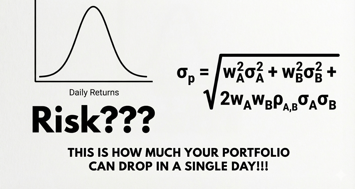
σ_p = √[ (w_A² × σ_A²) + (w_B² × σ_B²) + (2 × w_A × w_B × ρ_{A,B} × σ_A × σ_B) ]
Worked Example: Consider a portfolio with the following characteristics:
Asset X: 80% weight (w_X = 0.8), 16% standard deviation (σ_X = 0.16)
Asset Y: 20% weight (w_Y = 0.2), 25% standard deviation (σ_Y = 0.25)
Correlation: ρ_{X,Y} = 0.6
Using the first formula for variance:
σ_p² = (0.8)²(0.16)² + (0.2)²(0.25)² + 2(0.8)(0.2)(0.6)(0.16)(0.25)σ_p² = 0.016384 + 0.0025 + 0.00768σ_p² = 0.026564 (or 2.66%)
For standard deviation:
σ_p = √(0.026564) = 0.163or 16.3%
2.4. Scaling to Reality: The N-Asset Portfolio (Matrix Form)
The two-asset formula is essential for teaching, but real-world portfolios contain hundreds of assets. Professionals use matrix algebra to handle this complexity.
The formula expands rapidly. For 3 assets (A, B, C), the variance formula becomes:
σ_p² = w_A²σ_A² + w_B²σ_B² + w_C²σ_C² + 2w_A w_B Cov(A,B) + 2w_A w_C Cov(A,C) + 2w_B w_C Cov(B,C)
This portfolio has 3 variance terms and 3 covariance terms. A 100-asset portfolio would have 100 variance terms but (100 × 99) / 2 = 4,950 unique covariance terms.
This mathematical fact reveals the most important concept in large portfolios: as the number of assets (N) increases, the number of covariance terms grows exponentially faster (≈ N²) than the number of variance terms (N).
For a large, diversified portfolio, the individual, standalone risks (variances) of the assets become almost irrelevant. The entire risk of the portfolio is dominated by the interaction terms—the average covariance or correlation among all assets in the portfolio.
To manage this, the generalized N-asset formula is expressed in matrix notation:
σ_p² = w^T × Σ × w
Where:
wis a column vector (N x 1) of the weights of all assets.w^Tis the transpose (a 1 x N row vector) of the weights.Σ(Sigma) is the Variance-Covariance Matrix.
The Variance-Covariance Matrix (Σ) is an N x N matrix that organizes all the risk information for the portfolio. The elements on the main diagonal (top-left to bottom-right) are the variances (σ_A², σ_B², etc.) of each individual asset. All off-diagonal elements are the covariances (Cov(A,B), Cov(A,C), etc.) between each pair of assets.
This matrix is the complete set of risk inputs required for calculating the variance of an N-asset portfolio.
Part 3: The Bell Curve and Its 68-95-99.7 Promise
This section bridges the gap between the calculated risk statistic (portfolio standard deviation, σ_p) and the probability of specific gains or losses.
3.1. The “Normal” Assumption in Finance
The “Bell Curve,” known formally as the Normal Distribution, is a statistical distribution that is symmetric around its mean. Data points are most frequent at the mean, and become progressively rarer the further they are from the mean.
A foundational assumption in MPT, as well as in other critical financial models like the Black-Scholes option pricing formula, is that stock returns are normally distributed.
The implication of this assumption is profound. If returns are “normal,” they tend to cluster near the average. Extreme deviations, such as massive single-day gains or catastrophic losses, are modeled as being exceptionally rare. This assumption is what allows for the elegant and simple risk modeling that follows, as it suggests market behavior is, for the most part, predictable and contained.
3.2. The Empirical Rule (The 68-95-99.7 Rule)
This rule is the statistical shorthand for understanding the probabilities associated with a normal distribution. It is also known as the three-sigma rule.
It states that for any normally distributed data:
One Standard Deviation (± 1σ):
Approximately 68.27% of all data points (e.g., daily returns) will fall within one standard deviation of the mean (μ ± 1σ).
Interpretation: On a “normal” day, there is a ~68% probability that a portfolio’s return will be within its 1-sigma range.
Two Standard Deviations (± 2σ):
Approximately 95.45% of all data points will fall within two standard deviations of the mean (μ ± 2σ).
Interpretation: This range is considered to contain all highly probable outcomes. Only about 4.6% of all trading days should ever fall outside this range.
Three Standard Deviations (± 3σ):
Approximately 99.73% of all data points will fall within three standard deviations of the mean (μ ± 3σ).
Interpretation: This range is expected to capture almost all data. A “3-sigma event” (a return beyond this range) is considered exceptionally rare.
3.3. One-Sided Probabilities: “How Much Can I Lose?”
The Empirical Rule is two-sided (capturing both gains and losses). However, as investors, risk is generally perceived as the potential for loss. Because the Bell Curve is perfectly symmetric, we can divide the “outside” probabilities by two to find the probability of an extreme loss on one side.
Probability of a >1σ Loss: The 68.27% rule means 31.73% of data is outside the ± 1σ range. Due to symmetry, half of that (15.87%) lies above +1σ (large gain) and half (15.87%) lies below -1σ (large loss).
Probability of a loss greater than 1 standard deviation is 15.87%.
Probability of a >2σ Loss: The 95.45% rule means 4.55% of data is outside the ± 2σ range.
The probability of a loss greater than 2 standard deviations is half of that: 2.28%.
Probability of a >3σ Loss: The 99.73% rule means 0.27% of data is outside the ± 3σ range.
The probability of a loss greater than 3 standard deviations is 0.135%.
These probabilities can be translated into expected frequencies, which makes their implications much clearer:
± 1σ: Loss > X happens 1 in ~6 trading days.
± 2σ: Loss > X happens 1 in ~44 trading days.
± 3σ: Loss > X happens 1 in ~740 trading days (~3 years).
± 5σ: Loss > X happens 1 in ~3.5 million trading days.
This table highlights the core promise of the normal distribution: that a 2-sigma event is uncommon, a 3-sigma event is rare, and a 5-sigma event is so statistically improbable (once every 13,000+ years) as to be considered impossible. This assumption will be critically examined in Part 5.
Part 4: The Step-by-Step Guide: Estimating Your Portfolio’s Daily Movement
This section provides a practical, step-by-step guide that synthesizes the concepts from Parts 1, 2, and 3 to answer the central query: “how much can your portfolio of stock go up or down, in a day.”
Objective: To calculate the 1-standard-deviation (68% probability) and 2-standard-deviation (95% probability) ranges for a portfolio’s daily movement.
Step 1: Get Your Three Key Inputs To begin, one must have the following three pieces of data for all assets in the portfolio:
Asset Weights (w): The percentage (expressed as a decimal) of the total portfolio value allocated to each asset (e.g., w_A = 0.6, w_B = 0.4).
Asset Daily Standard Deviations (σ): The individual daily volatility for each asset, calculated as shown in Part 1.3.
Correlation Coefficients (ρ): The correlation coefficient between each pair of assets in the portfolio. This is a critical input that measures the diversification benefit.
Step 2: Calculate Your Portfolio’s Daily Standard Deviation (σ_p) The inputs from Step 1 must be combined using the portfolio variance formula. For this guide, a 2-asset portfolio (Asset A and Asset B) will be used.
Formula:
σ_p = √[ w_A²σ_A² + w_B²σ_B² + 2w_A w_B ρ_{A,B} σ_A σ_B ]
Worked Example (Hypothetical Portfolio):
Portfolio: 60% invested in Stock A (a tech stock) and 40% in Stock B (a utility stock).
Inputs:
Weights: w_A = 0.60, w_B = 0.40
Daily Volatility: σ_A = 2.0% (or 0.02), σ_B = 1.0% (or 0.01)
Correlation: ρ_{A,B} = 0.2 (low positive correlation)
Calculation:
Term for A:
(0.60)² × (0.02)² = 0.000144Term for B:
(0.40)² × (0.01)² = 0.000016Term for A,B (Interaction):
2 × (0.60) × (0.40) × (0.2) × (0.02) × (0.01) = 0.0000192Sum for Total Portfolio Variance (σ_p²):
0.0001792Calculate Portfolio Standard Deviation (σ_p):
√0.0001792 = 0.01338
Result: The portfolio’s daily standard deviation (volatility) is 1.34%.
Step 3: Establish Your Mean Expected Daily Return (μ) The Empirical Rule (Part 3) requires a mean (μ) and a standard deviation (σ). We now have σ_p.
For the mean, when calculating short-term (daily) risk, the expected mean return is statistically tiny compared to the daily volatility. For example, a 10% annual return averages to a daily log return of ln(1.10) / 252 ≈ 0.038%, which is dwarfed by the 1.34% volatility.
Therefore, it is standard practice—and provides a more conservative (pessimistic) risk estimate—to assume the mean daily return (μ) is 0.
Step 4: Apply the Empirical Rule (The Final Answer) Using the values derived above, we can now define the probable daily ranges for the portfolio:
Portfolio Daily Mean (μ) = 0%
Portfolio Daily Standard Deviation (σ_p) = 1.34%
1. The 1-Standard-Deviation (68%) Daily Range:
Formula:
μ ± 1σ_pCalculation:
0% ± (1 × 1.34%) = ± 1.34%Interpretation: Based on the normal distribution model, there is a 68% probability that this portfolio’s total return for the next trading day will fall within the range of -1.34% to +1.34%.
2. The 2-Standard-Deviation (95%) Daily Range:
Formula:
μ ± 2σ_pCalculation:
0% ± (2 × 1.34%) = ± 2.68%Interpretation: Based on the normal distribution model, there is a 95% probability that this portfolio’s total return for the next trading day will fall within the range of -2.68% to +2.68%.
This model provides a baseline for expectations. It implies that a day where the portfolio loses 3% is a “2-sigma event” (or rarer), which the model predicts should only occur about 1 in 44 trading days. This allows an investor to distinguish between a “normal” bad day and a “statistically significant” (tail) event.
Part 5: The “Deep Research” Critique – When the Bell Curve Fails
This section provides the essential expert-level nuance. The calculation in Part 4 is the academic foundation, but it is dangerously simplistic. Its conclusions are systematically wrong in the real world.
5.1. The Market is Not “Normal”
The central assumption of Parts 3 and 4—that financial returns are normally distributed—is empirically false. Real-world return distributions, when plotted, do not look like a perfect Bell Curve. They have two critical differences:
They have a much higher peak (more days of near-zero returns).
They have dramatically “fat tails”.
This phenomenon is called Leptokurtosis. It is the statistical term for a distribution with a high peak and “fat tails” (formally, a kurtosis value greater than 3). Financial returns are, by their nature, highly leptokurtic.
The “fat tails” are the most critical feature. It means that extreme events are not rare.
A “5-sigma” or “8-sigma” event, which the Bell Curve predicts should happen once in millions of years, has been observed to happen multiple times per decade in global financial markets. The 1987 “Black Monday” crash, the 2000 dot-com bubble, the 2008 financial crisis, and the 2020 COVID crash were all “fat tail” events.
The profound implication is that the models used in Part 4, which are built on the normal distribution, chronically and dangerously underestimate the probability and magnitude of market crashes.
5.2. The Flaws of Standard Deviation as a Risk Measure
Because standard deviation is the central component of a flawed “normal” model, it is an incomplete and often misleading measure of true risk.
It is Symmetrical (The “Upside” Problem): Standard deviation punishes all deviations from the mean, both positive and negative. It treats a +20% return (a massive gain) as equally “risky” as a -20% return (a massive loss). This is psychologically and financially absurd. Investors are not concerned with “upside volatility”; they are concerned with downside risk (the potential for loss).
It Underestimates Tail Risk: As established in 5.1, the “fat tails” of real markets mean that extreme losses are far more frequent than the 95% (2-sigma) or 99.7% (3-sigma) rules suggest. An investor who builds a portfolio to withstand a 2-sigma event will be completely unprepared for the real-world 5-sigma events that will happen. Real-world market crashes are these tail events.
It is a Historical, Not Predictive, Measure: Standard deviation is a descriptive statistic of past data. It is used to predict future risk based on the critical assumption that the future will resemble the past. This assumption breaks down violently during market regime changes and crises. The volatility in 2007 was no predictor for the volatility in 2008.
Part 6: A Better Tool – Value at Risk (VaR) and Conditional VaR (CVaR)
To address the profound failures of standard deviation, professionals developed more sophisticated, one-sided risk metrics that focus specifically on losses.
6.1. Value at Risk (VaR): The Industry Standard
Value at Risk (VaR) is a statistical measure that quantifies the maximum potential loss over a specific time horizon at a given confidence level. VaR answers a different, more useful question than standard deviation. It discards the “upside” and focuses only on the loss.
It answers, “What is the most I can expect to lose on 95% of days?”
Clear Interpretation:
Statement: “My portfolio has a 1-day, 95% VaR of $1 million.”
Meaning: This means that on 19 out of 20 trading days (95% confidence), the portfolio’s losses are expected to be less than $1 million.
The Tail: This also means that on 1 out of 20 trading days (a 5% probability), the portfolio’s losses are expected to be greater than $1 million.
Calculating VaR (Parametric Method): This common method still assumes a normal distribution (a flaw we will address), but it is a one-sided calculation. Instead of the 68-95-99.7 rule, it uses the specific Z-score from the normal distribution that corresponds to the chosen confidence level.
For 95% confidence (a 5% tail), the one-sided Z-score is 1.645.
For 99% confidence (a 1% tail), the one-sided Z-score is 2.33.
Formula: VaR_{95%} = μ - (1.645 × σ_p)
Using our Part 4 Example:
VaR_{95%} = 0% - (1.645 × 1.34%)VaR_{95%} = -2.20%
Interpretation: We are 95% confident that our portfolio will not lose more than 2.20% in a single day. This is a more precise and useful risk statement than the 2-sigma range of ± 2.68% calculated in Part 4.
6.2. The “But” of VaR: The 2008 Financial Crisis and the Flaw
VaR became the global standard for risk management in the 1990s and 2000s, but it is critically flawed for the same reason standard deviation is: it fails to account for fat tails.
The flaw in VaR is even more insidious. VaR tells you the minimum you will lose in a tail event, but it says nothing about the magnitude of that loss.
The VaR Catastrophe: A 95% VaR of -2.20% only tells you that on 5% of days, your loss will be worse than -2.20%. It is completely silent on the critical question: will that loss be -2.21% or -20%?
This analytical “blind spot” is what led to the collapse of firms like Long-Term Capital Management, which had optimized its portfolio to a VaR limit but was destroyed by a “fat tail” loss just beyond that limit. It was a primary reason so many banks were under-capitalized for the 2008 financial crisis. They were prepared for 99% VaR events, but not for the magnitude of the 1% “fat tail” events that actually occurred.
6.3. Conditional Value at Risk (CVaR): The Superior Metric
This is the modern, robust, expert-level solution. Conditional Value at Risk (CVaR), also known as Expected Shortfall (ES), Average VaR (AVaR), or Expected Tail Loss (ETL), was designed specifically to fix the fatal flaw of VaR.
Definition: CVaR explicitly measures the risk in the fat tail. It is the average expected loss that occurs conditional on that loss exceeding the VaR threshold.
The Question it Answers: CVaR answers the question VaR cannot: “When a tail event does happen (i.e., when my losses exceed the 95% VaR), what is my average expected loss?“
VaR vs. CVaR (The Definitive Insight):
VaR is the gate to the tail. It is the best-case scenario (i.e., minimum loss) in that tail.
CVaR is the average loss inside the tail. By definition, CVaR will always be a larger, more conservative number than VaR.
Why CVaR is Superior:
It Quantifies the Tail: It directly captures the “fat tail” risk that VaR and standard deviation ignore or are silent on. It provides a real number for the expected loss in a crisis.
It is “Coherent”: Unlike VaR, CVaR is a “coherent risk measure”. This is a technical term with a critical meaning: it is “subadditive.” This means the CVaR of a diversified portfolio will always be less than or equal to the sum of the CVaRs of its parts. It always correctly reflects the benefits of diversification, whereas VaR can, in some complex cases, fail to do so.
Because of its mathematical robustness and its ability to quantify tail risk, CVaR (or Expected Shortfall) is the true measure of downside risk. It is more conservative and has been adopted by global banking regulators (e.g., the Basel Committee on Banking Supervision) to replace VaR for determining banks’ regulatory capital requirements.
Conclusion: A Framework for Intelligent Risk Analysis
This article has provided a deep, quantitative dive into “portfolio variation.” The analysis has progressed through the entire arc of modern risk management, from its genesis with Markowitz’s Nobel Prize-winning work to its catastrophic failures during the 2008 financial crisis and the superior, more robust metrics that have emerged in its wake.
The key takeaways from this research are as follows:
Risk is Interaction: The central mechanism of portfolio risk is not individual volatility, but correlation. Diversification is the only “free lunch” in finance, and its mathematical engine is the combination of assets with low or negative correlation to reduce total portfolio variance.
The Model is a Starting Point: A full, step-by-step guide (Part 4) to calculate the 1-sigma (68%) and 2-sigma (95%) daily ranges for a portfolio has been provided, as requested. This calculation represents the academic answer to the query and is the foundation of MPT.
The Model is Wrong: The expert answer is that this model is built on the provably false assumption of a “Bell Curve”. Real financial markets have “fat tails”. This means the simple model in Part 4 will fail during a crisis by systematically underestimating the probability and magnitude of catastrophic losses.
Ask the Right Question: An intelligent analysis of risk requires moving beyond the flawed, symmetrical question, “What is my volatility?” Investors must ask the more precise, one-sided questions that professionals now use:
Value at Risk (VaR): “What is the minimum I can expect to lose in a tail event?”
Conditional VaR (CVaR): “When that tail event happens, what is my average expected loss?”
By framing an analysis around this narrative—from the simple model, to its critical flaws, to the superior solutions—one can achieve a truly expert-level, nuanced, and actionable understanding of portfolio risk.
Do not stop at the simple math. Dig deeper until you find the model that accounts for the hard reality of the market.
All the best,
Nicolau
Creator and Author of the Technical Intrinsic Value Model
*Disclaimer: This is for educational purposes based on a personal investment. It is not financial advice. Past performance is not indicative of future results. All investments involve risk.*